Figure 11

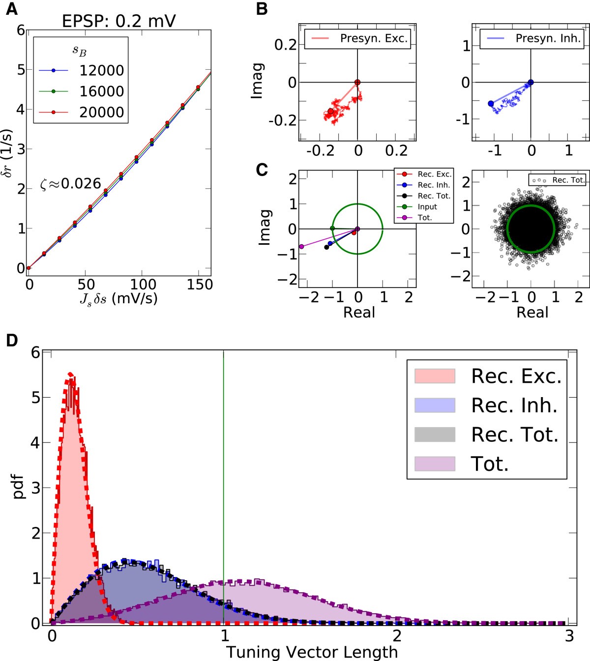
Linear tuning in recurrent networks. (A) Linearized gains for single neurons embedded in the network. The extra firing rate, δ r, of a neuron produced in response to a small perturbation, J _s δ s, in the input intensity, plotted for different baseline inputs corresponding to different contrasts. The response is computed by numerically perturbing the mean-field equations (see Methods). The linear gain, ζ=δ r/(J _s δ s), is then computed by linear regression of data points. For this example with EPSP = 0.2 mV, the value ζ = 0.026 is obtained, which is also used for the next panels. (B) For the sample neuron in Figure 2A, all presynaptic Tuning Vectors are extracted ($J\text{exp}\left(j2\underset{i}{\overset{\ast }{\theta }}\right)$, weighted by the linear gain (ζ), and vectorially added together, reflecting linear integration in neurons. Although each presynaptic vector makes only a small contribution, the resulting random sum can lead to a large resultant Tuning Vector. These are generally larger for presynaptic inhibition (Presyn. Inh.) compared to presynaptic excitation (Presyn. Exc.). Note different scales of axes. (C) Left panel: The resultant vectors for recurrent excitation (Rec. Exc.), recurrent inhibition (Rec. Inh.), total recurrent (Rec. Tot. = Rec. Exc. + Rec. Inh.), feedforward input (Input), and the total input (Tot. = Input + Rec. Tot.) are plotted. All normalized input Tuning Vectors have the same length of one, denoted by the green circle. Right panel: Total recurrent Tuning Vectors (Rec. Tot.) for all neurons in the network are compared with the normalized length of their input Tuning Vectors (green circle). D) Distribution of the length of all Tuning Vectors for all the neurons in the network. Dashed lines show the predicted distributions of the linear analysis in each case (see text for details).